Creating our new type of Riemann sum (part 1)
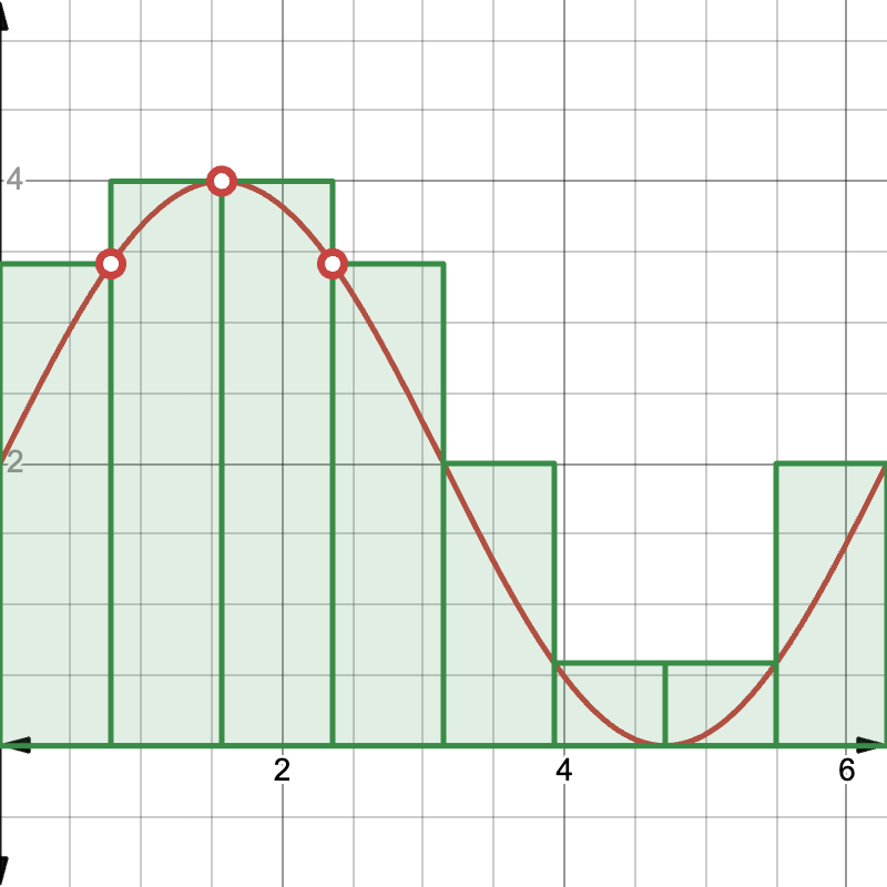
Let’s say we want to find the area under the function \(f(x) = 2\sin(x) + 2\) over the interval \([0, 2\pi]\). As an example, we can divide the interval into 8 equal subintervals:
Slide 1 (can use arrow keys to navigate; press "t" for timer, "f" to go to first slide, "l" to go to last slide, or "h" to show/hide this UI)
Introduction
Hello! This is a presentation about Riemann integration that I presented to some of my college friends on February 11, 2025.
Instead of making a boring slideshow, I decided to make an interactive website for my presentation!
This is my second time making an interactive presentation! The first time was for my high school’s math club, and you can view the presentation here:
MATH 2117 Lecture 1: Riemann Integration Explained Simply
Like MATH 2417, but betterTM
By Eldrick Chen / calculus gaming
Creator of unnamed calc website and other related websites
# of Rectangles =
Riemann sums
A way to approximate the area under a curve
Example: Right Riemann sums for \(f(x) = x^2\) on the interval \([0, 2]\)
# of Rectangles =
Area ≈
The not-so-rigorous definition of an integral
In English: the area under \(f(x)\) from \(x=a\) to \(x=b\) is the limit of a Riemann sum (in this case, a right Riemann sum) as the number of rectangles approaches infinity.
It works most of the time, but some weird functions can cause problems...
After all, we’re only doing one specific type of Riemann sum here - a right Riemann sum. What if we did the Riemann sum some other way? Would we still get the same area?
Let’s make this more rigorous!
We want to prove that any possible Riemann sum will approach the same area as we make the rectangles smaller.
To do that, we can consider, given a partition (a specific way of dividing an interval):
As we decrease the width of the rectangles, hopefully the maximum possible Riemann sum and minimum possible Riemann sum will approach the same number. In that case, we can confidently say that that number is the area under the curve!
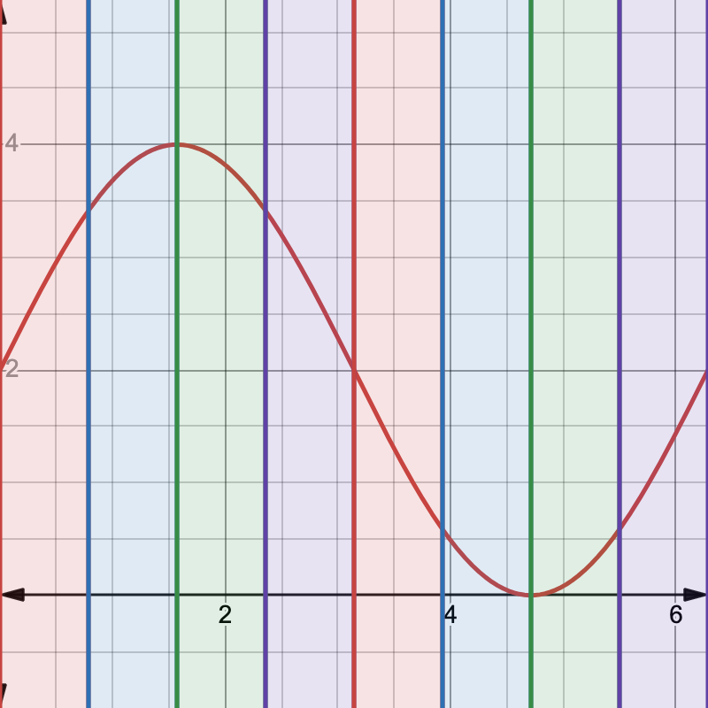
Creating our new type of Riemann sum (part 1)
Let’s say we want to find the area under the function \(f(x) = 2\sin(x) + 2\) over the interval \([0, 2\pi]\). As an example, we can divide the interval into 8 equal subintervals:
Creating our new type of Riemann sum (part 2)
In a standard calculus class, you probably learned about left and right Riemann sums, where the height of each rectangle is determined by evaluating the function at the left or right boundary of each subinterval.
We’re going to do something different: we’re going to introduce the upper and lower Riemann sums. Let’s try having the height of each rectangle be determined by the maximum or minimum value the function takes on within each subinterval.
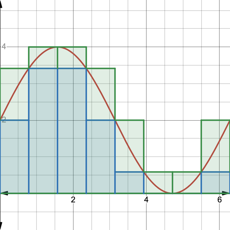
The blue rectangles represent a lower Riemann sum, and the green rectangles represent an upper Riemann sum by our current definition.
A small problem with our definition
Our current definition works well for continuous functions, but we encounter an issue with discontinuous functions. Consider this function:
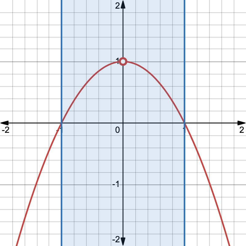
What is the maximum of this function on the interval \([-1, 1]\) (the blue shaded region)?
Finding the maximum of this discontinuous function
\(y = \)
What’s going on?
As it turns out, this function does not have a maximum on \([-1, 1]\). However, the number 1 still feels somehow related to this function. It’s like we want to say the maximum is 1 but we can’t because of the technicality that \(f(x)\) doesn’t actually reach \(y = 1\). After all, \(f(x)\) can become arbitrarily close to 1, it just can’t actually reach 1.
To fix this, we need a new concept that’s related to the maximum but can account for scenarios like this where the function can become arbitrarily close to the value, but never actually reach it.
Introducing: THE SUPREMUM
The concept that fixes this problem is known as the supremum. To explain what this is, I first need to explain upper bounds.
An upper bound is a number that is greater than or equal to all numbers in a set. For example, 4 is an upper bound of the set \(\{1, 2, 3\}\) because 4 is greater than or equal to all numbers in that set.
Sets can have multiple upper bounds. For example, 3, 5, and 11 all also serve as upper bounds for the set \(\{1, 2, 3\}\).
Visualizing upper bounds (part 1)
Here’s the function from before, except without the discontinuity.
\(y = \)
Visualizing upper bounds (part 2)
Now let’s add back the discontinuity:
\(y = \)
How upper bounds relate to the supremum
The supremum is defined as the smallest possible upper bound for a set.
\(y = \)
Definitions of supremum and infimum
A supremum (abbreviated \(\sup\)) is the smallest possible upper bound for a set. It is similar to a maximum, but sometimes the supremum of a set can exist even if the maximum doesn’t.
An infimum (abbreviated \(\inf\)) is the largest possible lower bound for a set. It is similar to a minimum, but sometimes the infimum of a set can exist even if the minimum doesn’t.
Revising our definition of upper/lower Riemann sums (part 1)
Let’s go back to our previous upper/lower Riemann sum example, where we were trying to find the area under \(f(x) = 2\sin(x) + 2\) over \([0, 2\pi]\) using 8 equal subintervals.
By our previous definition, we defined the height of each rectangle to be the maximum/minimum value the function takes on within each subinterval.
The blue rectangles represent a lower Riemann sum, and the green rectangles represent an upper Riemann sum by our previous definition (using maximum/minimum).
Revising our definition of upper/lower Riemann sums (part 2)
Our previous definition can fail for functions that don’t attain a maximum/minimum over certain intervals.
To fix this, we instead can use the supremum and infimum to define upper and lower Riemann sums.
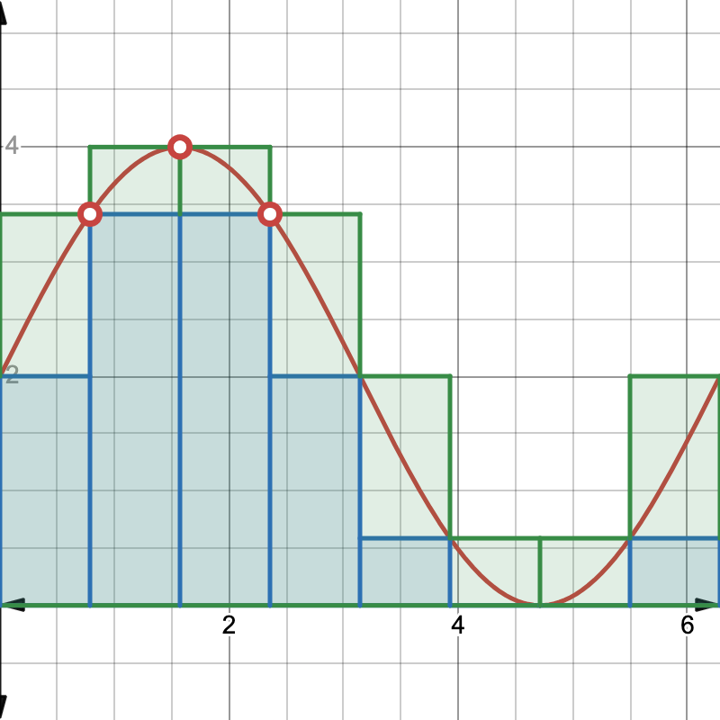
The blue rectangles represent a lower Riemann sum, and the green rectangles represent an upper Riemann sum by our current definition (using supremum/infimum).
A note on terminology
We’re almost ready to actually go over the formal definition of Riemann integration now, but there is one more thing to note:
“Riemann integration” can actually refer to one of two things!
These are two different ways to rigorously define integrals, but luckily, they are equivalent (they always give the same results). I’ll be going over Darboux integrals in this presentation.
What is a partition?
A partition is an ordered collection of points within an interval \([a, b]\) that also includes the endpoints.
Here’s the formal definition: A partition \(P\) of \([a, b]\) is a set \(P = \{a = t_0 \lt t_1 \lt t_2 \lt \cdots \lt t_n = b\}\).
For example, the set \(\{t_0 = \class{red}{1}, t_1 = 1.2, t_2 = 1.7, t_3 = \class{blue}{2}\}\) is a partition of the interval \([\class{red}{1}, \class{blue}{2}]\).
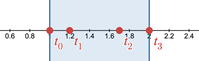
A visualization of the above partition. The red points are part of the partition, and the blue region represents the interval \([1, 2]\).
Partitions and subintervals
A partition essentially functions as a way to divide an interval into multiple smaller intervals (subintervals).
For example, using the partition of \([1, 2]\) from before, \(\{\class{red}{1}, \class{green}{1.2}, \class{purple}{1.7}, \class{blue}{2}\}\), we can create 3 subintervals: \([\class{red}{1}, \class{green}{1.2}]\), \([\class{green}{1.2}, \class{purple}{1.7}]\), and \([\class{purple}{1.7}, \class{blue}{2}]\).
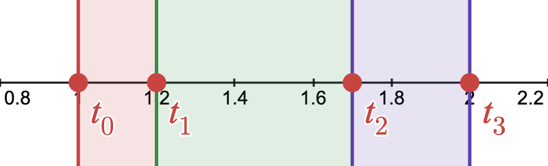
A visualization of the 3 subintervals created by this partition.
Notice that the subintervals in this case are \(\class{red}{[t_0, t_1]}\), \(\class{green}{[t_1, t_2]}\), and \(\class{purple}{[t_2, t_3]}\).
In general, for a partition \(\{a = t_0 \lt t_1 \lt t_2 \lt \cdots \lt t_n = b\}\) of the interval \([a, b]\), the corresponding subintervals are \([t_0, t_1]\), \([t_1, t_2]\), ..., \([t_{n-1}, t_n]\).
Finding a formula for the area of each rectangle (part 1)
Let’s look at this upper Riemann sum.
What is the height of each rectangle?
The height of the 1st rectangle is the supremum of \(f(x)\) over \([t_0, t_1]\).
The height of the 2nd rectangle is the supremum of \(f(x)\) over \([t_1, t_2]\).
The height of the 3rd rectangle is the supremum of \(f(x)\) over \([t_2, t_3]\).
In general, the height of the \(i\)th rectangle is the supremum of \(f(x)\) over \([t_{i-1}, t_{i}]\).
Finding a formula for the area of each rectangle (part 2)
What is the width of each rectangle?
The width of the 1st rectangle is \(t_1 - t_0\).
The width of the 2nd rectangle is \(t_2 - t_1\).
The width of the 3rd rectangle is \(t_3 - t_2\).
In general, the width of the \(i\)th rectangle is \(t_{i-1} - t_{i}\).
Finding a formula for the area of each rectangle (part 3)
What is the area of each rectangle? Here’s what we’ve figured out:
The height of the \(i\)th rectangle is the supremum of \(f(x)\) over \([t_{i-1}, t_{i}]\). Let’s call this value \(M_i\).
The width of the \(i\)th rectangle is \(t_{i-1} - t_{i}\). So the area of the \(i\)th rectangle is:
A formula for the upper sum
Let \(f(x)\) be bounded on \([a, b]\). Suppose \(P\) is a partition of \([a, b]\). Then the upper Darboux sum corresponding to \(P\) is defined as:
Where \(M_i\) (the height of the \(i\)th rectangle) is defined as:
Remember that \(M_i(t_{i-1} - t_i)\) is the area of the \(i\)th rectangle. So this expression is just summing up the areas of all rectangles.
A formula for the lower sum
Let \(f(x)\) be bounded on \([a, b]\). Suppose \(P\) is a partition of \([a, b]\). Then the lower Darboux sum corresponding to \(P\) is defined as:
Where \(m_i\) (the height of the \(i\)th rectangle) is defined as:
This is the same as the upper sum, except we’ve replaced the supremum with an infimum.
The upper Darboux integral (part 1)
Upper Darboux sums typically get more accurate as you increase the number of rectangles. So how do we find the actual area under the curve?
Upper Darboux sums overestimate the area under the curve, so as they get more accurate, the area decreases. So to find the area under the curve, it seems like we should find the lowest possible upper Darboux sum.
# of Rectangles =
Area ≈
In this case, the upper Darboux sum typically decreases as we add more rectangles. The smaller the sum is, the closer it is to the true sum!
The upper Darboux integral (part 2)
So you might think that we can just take the minimum value of all possible upper Darboux sums. Except there’s a problem: what if the upper Darboux sums can become arbitrarily close to the true area, but never actually approach it? In other words, what if the upper Darboux sum will always overestimate the area by some amount, even though we can make that amount arbitrarily small?
The upper Darboux integral (part 3)
To fix this, we instead find the infimum of all possible upper Darboux sums - the highest possible lower bound. This is known as the upper Darboux integral.
You can think of the upper Darboux integral as the limit to how small we can make the upper Darboux sums (i.e. it is impossible to construct an upper Darboux sum with a value smaller than the upper Darboux integral).
The lower Darboux integral
The lower Darboux integral is very similar to the upper Darboux integral, except we’re now finding the supremum of all possible lower Darboux sums.
You can think of the lower Darboux integral as the limit to how large we can make the lower Darboux sums (i.e. it is impossible to construct a lower Darboux sum with a value larger than the lower Darboux integral).
# of Rectangles =
Area ≈
Underestimates true area by about
The Darboux integral
If the upper and lower Darboux integrals are equal, then we call that value the Darboux integral of \(f(x)\) from \(x = a\) to \(x = b\). (Note that the “actual” Riemann integral, which is defined differently, will always be equal to the Darboux integral if it exists.)
A function is called Darboux integrable if this Darboux integral can be found, i.e. the upper and lower Darboux integrals exist and are equal. (A function is Riemann integrable if and only if it is Darboux integrable.)
A function \(f(x)\) is Darboux/Riemann integrable if and only if:
For every \(\epsilon \gt 0\), there is a partition \(P\) such that \(U(P, f) - L(P, f) \lt \epsilon\).
In other words, we can make the upper and lower Darboux sums arbitrarily close to each other by choosing partitions in some way (typically by making the subintervals smaller and smaller).
The Darboux integral: an interactive example
# of Rectangles =
Upper Darboux sum ≈
Lower Darboux sum ≈
Upper Darboux sum - lower Darboux sum ≈
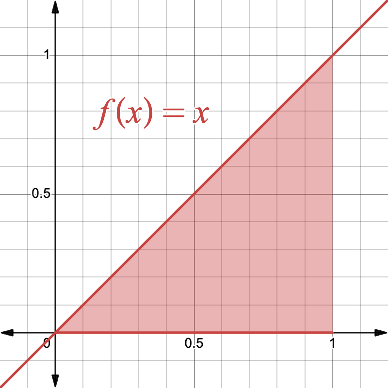
The Darboux integral: a simple example
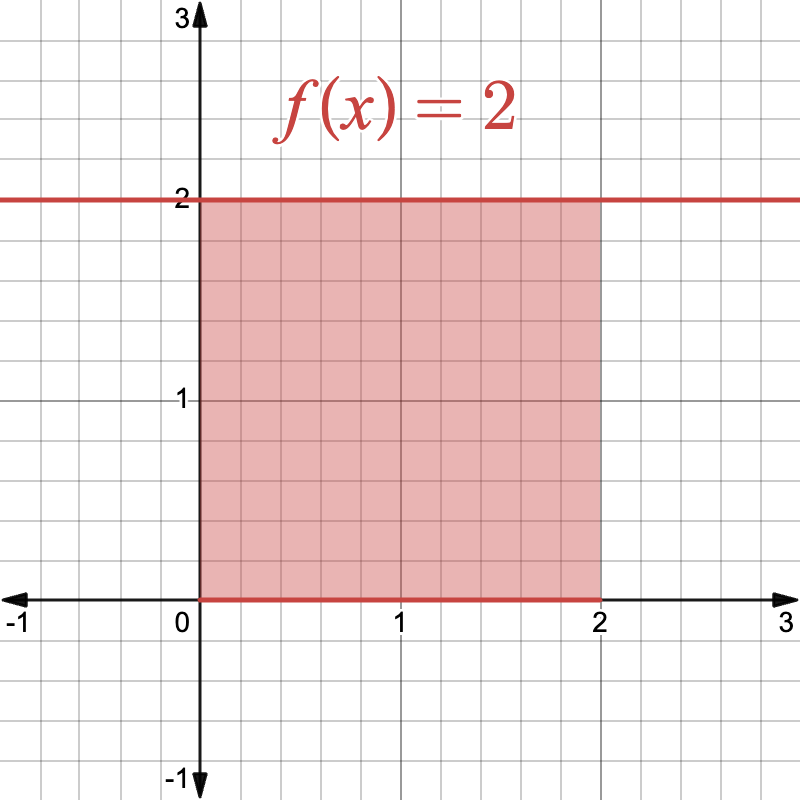
Let’s start off with a simple example:
How would we find this integral using the formal definition?
The Darboux integral: a simple example
Let \(P = \{0 = t_0 \lt t_1 \lt \cdots \lt t_n = 2\}\) be an arbitrary partition of \([0, 2]\).
Because \(f(x) = 2\) is constant, the supremum over any interval \([t_{i-1}, t_i]\) is 2.
Similarly, the infimum over any interval \([t_{i-1}, t_i]\) is 2.
The Darboux integral: a simple example
Now let’s find the upper Darboux sum:
Any upper Darboux sum of \(f(x) = 2x\) over \([0, 2]\) is equal to 4. Therefore:
The Darboux integral: a simple example
Now let’s find the lower Darboux sum:
Any lower Darboux sum of \(f(x) = 2x\) over \([0, 2]\) is equal to 4. Therefore:
Because the upper Darboux integral (4) is equal to the lower Darboux integral (4), the overall Darboux integral of \(f(x) = 2x\) over \([0, 2]\) is equal to 4.
The Darboux integral: a simple example
# of Rectangles =
Upper Darboux sum = 4
Lower Darboux sum = 4
Upper Darboux sum - lower Darboux sum = 0
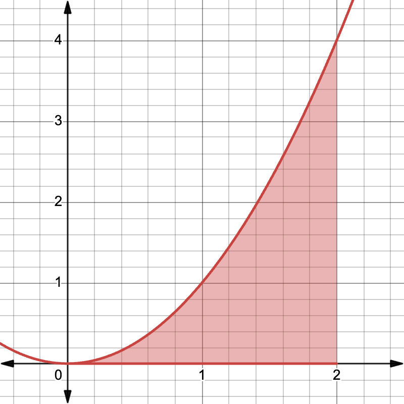
The Darboux integral: a harder example
Let’s say we want to find the following integral:
How would we do so using the formal definition?
The Darboux integral: a harder example
Let \(P_n = \{0 = t_0 \lt t_1 \lt t_2 \lt \cdots \lt t_n = 1\}\), where \(t_i = \frac{i}{n}\). Therefore, \(t_i - t_{i-1} = \frac{1}{n}\).
In simple words, the partition \(P_n\) divides the interval \([0, 1]\) into \(n\) equal subintervals.
# of Rectangles (\(n\)) =
The Darboux integral: a harder example
This is the value of the upper Darboux sum using \(n\) equal subintervals.
The Darboux integral: a harder example
# of Rectangles (\(n\)) =
Upper Darboux sum ≈
The Darboux integral: a harder example
This is the value of the lower Darboux sum using \(n\) equal subintervals.
The Darboux integral: a harder example
# of Rectangles (\(n\)) =
Lower Darboux sum ≈
The Darboux integral: a harder example
Here are the formulas we found for the upper and lower Darboux sums:
Because \(U(P_n, f)\) can become arbitrarily close to \(\frac{1}{2}\), the upper Darboux integral \(\inf\{U(P, f): P \text{ is a partition of } [a, b] \}\) must be at most \(\frac{1}{2}\). Similarly, the lower Darboux integral \(\sup\{L(P, f): P \text{ is a partition of } [a, b] \}\) must be at least \(\frac{1}{2}\). Because the upper Darboux integral must be greater than or equal to the lower Darboux integral, they both must be equal to \(\frac{1}{2}\).
So the Darboux integral \(\displaystyle\int_0^1 x\dd{x}\) is equal to \(\displaystyle\frac{1}{2}\).
The Darboux integral: a harder example
# of Rectangles =
Upper Darboux sum ≈
Lower Darboux sum ≈
Upper Darboux sum - lower Darboux sum ≈
The Darboux integral: the Dirichlet function
The Dirichlet function is an interesting function that basically tells you whether its input is rational or not. It is defined as follows:
Here are some examples:
The Darboux integral: the Dirichlet function
Here is my best attempt at graphing this function:
This graph is very misleading - this function is continuous nowhere, and this graph doesn’t even look like a function! However, it will still be useful for visualizing the Darboux sums for this function.
The Darboux integral: the Dirichlet function
What is the Darboux integral of the Dirichlet function over \([0, 1]\)?
Let \(P = \{0 = t_0 \lt t_1 \lt \cdots \lt t_n = 1\}\) be an arbitrary partition of \([0, 1]\).
Since any interval \([t_{i-1}, t_i]\) contains rational numbers, the supremum of \(f(x)\) over this interval is 1.
Since any interval \([t_{i-1}, t_i]\) also contains irrational numbers, the infimum of \(f(x)\) over this interval is 0.
The Darboux integral: the Dirichlet function
Let’s find the upper Darboux sum:
Any upper Darboux sum of the Dirichlet function over \([0, 1]\) is equal to 1. Therefore:
The Darboux integral: the Dirichlet function
Let’s find the lower Darboux sum:
Any lower Darboux sum of the Dirichlet function over \([0, 1]\) is equal to 0. Therefore:
Because the upper Darboux integral (1) isn’t equal to the lower Darboux integral (0), the Dirichlet function is not Riemann integrable over \([0, 1]\)! (In fact, it isn’t Riemann integrable over any interval.)
The Darboux integral: the Dirichlet function
# of Rectangles =
Upper Darboux sum = 1
Lower Darboux sum = 0
Upper Darboux sum - lower Darboux sum = 1
Quick summary of Darboux integrals
We want to find the exact area under a curve.
Quick summary of Darboux integrals
To do so, we create the idea of upper and lower Darboux sums, which respectively overestimate and underestimate the true area under the curve. We use the concepts of supremum and infimum to determine the height of each rectangle.
# of Rectangles =
Upper Darboux sum ≈
Lower Darboux sum ≈
Quick summary of Darboux integrals
To show that a function is Darboux/Riemann integrable, we need to show that the upper and lower Darboux sums can become arbitrarily close to each other. If so, the integral is equal to the value that both sums approach as they approximate the area more and more accurately.
# of Rectangles =
Upper Darboux sum ≈
Lower Darboux sum ≈
Upper Darboux sum - lower Darboux sum ≈
Thanks everyone!
Visit my website at https://calculusgaming.com for more educational content by calculus gaming!